Jupyter Notebook#

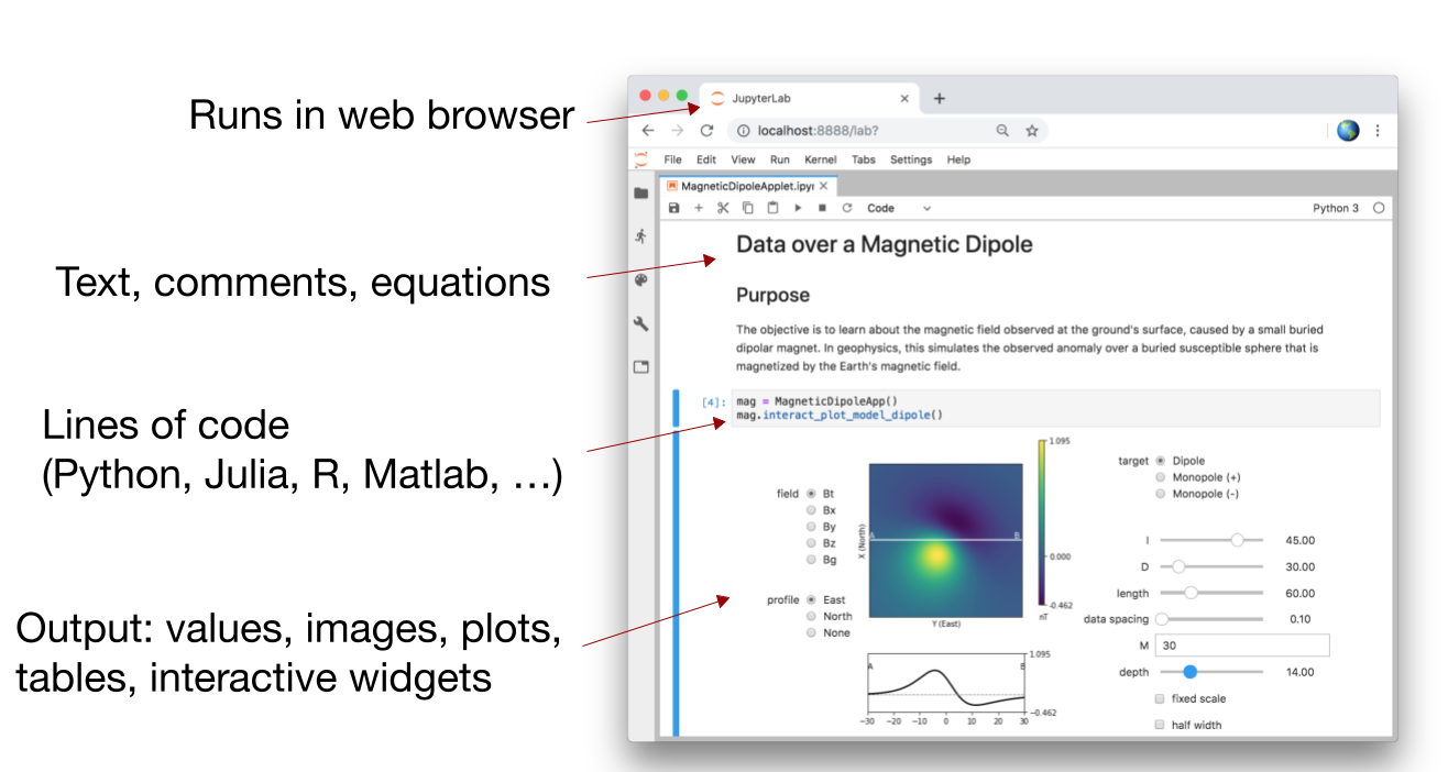
The Jupyter Notebook is an interactive computing environment that enables users to author notebook documents that include:

Live code
Interactive widgets
Plots
Narrative text
Equations
Images
Video

Notebook

These documents provide a complete and self-contained record of a computation that can be converted to various formats and shared with others using email, Dropbox, version control systems (like git/GitHub) or nbviewer.ipython.org.

Additional resources

JupyterLab documentation

This material is adapted from the ICESat2 Hackweek intro-jupyter-git session by @fperez.

Components#

The Jupyter Notebook combines three components:

The notebook web application
Kernels
Notebook documents

Notebook web application#

The notebook web application enables users to:

Edit code in the browser, with automatic syntax highlighting, indentation, and tab completion/introspection.
Run code from the browser, with the results of computations attached to the code which generated them.
See the results of computations with rich media representations, such as HTML, LaTeX, PNG, SVG, PDF, etc.
Create and use interactive JavaScript wigets, which bind interactive user interface controls and visualizations to reactive kernel side computations.
Author narrative text using the Markdown markup language.
Build hierarchical documents that are organized into sections with different levels of headings.
Include mathematical equations using LaTeX syntax in Markdown, which are rendered in-browser by MathJax.

Kernels#

Simply put, the kernel is the engine that runs the code. Each kernel is capable of running code in a single programming language and there are kernels available in over 100 programming languages.

IPython is the default kernel, it runs Python code.

Notebook documents#

Notebook documents contain the inputs and outputs of an interactive session as well as narrative text that accompanies the code but is not meant for execution. Rich output generated by running code, including HTML, images, video, and plots, is embeddeed in the notebook, which makes it a complete and self-contained record of a computation.

When you run the notebook web application on your computer, notebook documents are just files on your local filesystem with a .ipynb extension. This allows you to use familiar workflows for organizing your notebooks into folders and sharing them with others using email, Dropbox and version control systems.

Notebooks consist of a linear sequence of cells. There are three basic cell types:

Code cells: Input and output of live code that is run in the kernel
Markdown cells: Narrative text with embedded LaTeX equations
Raw cells: Unformatted text that is included, without modification, when notebooks are converted to different formats using nbconvert

Notebooks can be exported to different static formats including HTML, reStructeredText, LaTeX, PDF, and slide shows using Jupyter’s nbconvert utility.

Furthermore, any notebook document available from a public URL on or GitHub can be shared via http://nbviewer.jupyter.org. This service loads the notebook document from the URL and renders it as a static web page. The resulting web page may thus be shared with others without their needing to install Jupyter.

Body#

The body of a notebook is composed of cells. Each cell contains either markdown, code input, code output, or raw text. Cells can be included in any order and edited at-will, allowing for a large ammount of flexibility for constructing a narrative.

Markdown cells - These are used to build a nicely formatted narrative around the code in the document. The majority of this lesson is composed of markdown cells.
Code cells - These are used to define the computational code in the document. They come in two forms: the input cell where the user types the code to be executed, and the output cell which is the representation of the executed code. Depending on the code, this representation may be a simple scalar value, or something more complex like a plot or an interactive widget.
Raw cells - These are used when text needs to be included in raw form, without execution or transformation.

print("I'm a code cell!")

I'm a code cell!

Modality#

The notebook user interface is modal. This means that the keyboard behaves differently depending upon the current mode of the notebook. A notebook has two modes: edit and command.

Edit mode is indicated by a blue cell border and a prompt showing in the editor area. When a cell is in edit mode, you can type into the cell, like a normal text editor.

edit mode

Command mode is indicated by a grey cell background. When in command mode, the structure of the notebook can be modified as a whole, but the text in individual cells cannot be changed. Most importantly, the keyboard is mapped to a set of shortcuts for efficiently performing notebook and cell actions. For example, pressing c when in command mode, will copy the current cell; no modifier is needed.

command mode

Enter edit mode by pressing Enter or using the mouse to click on a cell’s editor area.

Enter command mode by pressing Esc or using the mouse to click outside a cell’s editor area.

Do not attempt to type into a cell when in command mode; unexpected things will happen!

import numpy as np

Mouse navigation#

The first concept to understand in mouse-based navigation is that cells can be selected by clicking on them. The currently selected cell is indicated with a blue outline or gray background depending on whether the notebook is in edit or command mode. Clicking inside a cell’s editor area will enter edit mode. Clicking on the prompt or the output area of a cell will enter command mode.

The second concept to understand in mouse-based navigation is that cell actions usually apply to the currently selected cell. For example, to run the code in a cell, select it and then click the button in the toolbar or the Run -> Run Selected Cells menu item. Similarly, to copy a cell, select it and then click the button in the toolbar or the Edit -> Copy menu item. With this simple pattern, it should be possible to perform nearly every action with the mouse.

Markdown cells have one other state which can be modified with the mouse. These cells can either be rendered or unrendered. When they are rendered, a nice formatted representation of the cell’s contents will be presented. When they are unrendered, the raw text source of the cell will be presented. To render the selected cell with the mouse, click the button in the toolbar or the Run -> Run Selected Cells menu item. To unrender the selected cell, double click on the cell.

Keyboard Navigation#

The modal user interface of the Jupyter Notebook has been optimized for efficient keyboard usage. This is made possible by having two different sets of keyboard shortcuts: one set that is active in edit mode and another in command mode.

The most important keyboard shortcuts are Enter, which enters edit mode, and Esc, which enters command mode.

In edit mode, most of the keyboard is dedicated to typing into the cell’s editor. Thus, in edit mode there are relatively few shortcuts. In command mode, the entire keyboard is available for shortcuts, so there are many more possibilities.

The following shortcuts have been found to be the most useful in day-to-day tasks:

Basic navigation:

enter: Enter edit mode
shift-enter: run cell
up/k, down/j: Move to cell above/below

Saving the notebook: s
Cell types:

y: code
m: markdown
r: raw

Cell creation:

a: create new cell above current cell
b: create new cell below current cell

Cell editing:

x: cut
c: copy
v: paste
d: delete (press twice)
z: redo

Kernel operations (press twice):

i: interrupt kernel
0: restart kernel

You can fully customize JupyterLab’s keybindings by accessing the Settings -> Advanced Settings Editor menu item.

Running Code#

First and foremost, the Jupyter Notebook is an interactive environment for writing and running code. Jupyter is capable of running code in a wide range of languages. However, this notebook, and the default kernel in Jupyter, runs Python code.

Code cells allow you to enter and run Python code#

Run a code cell using Shift-Enter or pressing the button in the toolbar above:

a = 10

print(a + 1)

Note the difference between the above printing statement and the operation below:

a + 1

a + 2

b = _

When a value is returned by a computation, it is displayed with a number, that tells you this is the output value of a given cell. You can later refer to any of these values (should you need one that you forgot to assign to a named variable). The last three are available respectively as auto-generated variables called _, __ and ___ (one, two and three underscores). In addition to these three convenience ones for recent results, you can use _N, where N is the number in [N], to access any numbered output.

There are two other keyboard shortcuts for running code:

Alt-Enter runs the current cell and inserts a new one below.
Note that Alt refers to the Option key on Macs. Make sure your browser settings do not intefere with the use of the Option key when using this shortcut.
Ctrl-Enter run the current cell and enters command mode.
Notice Shift-Enter runs the current cell and selects the cell below, while Ctrl-Enter stays on the executed cell in command mode.

Managing the IPython Kernel#

Code is run in a separate process called the IPython Kernel. The Kernel can be interrupted or restarted. Try running the following cell and then hit the button in the toolbar above.

import time
time.sleep(10)

If the Kernel dies you will be prompted to restart it. Here we call the low-level system libc.time routine with the wrong argument via ctypes to segfault the Python interpreter. To test it out, uncomment the next cell.

# import sys
# from ctypes import CDLL
# # This will crash a Linux or Mac system
# # equivalent calls can be made on Windows
# dll = 'dylib' if sys.platform == 'darwin' else 'so.6'
# libc = CDLL("libc.%s" % dll) 
# libc.time(-1)  # BOOM!!

Restarting the kernels#

The kernel maintains the state of a notebook’s computations. You can reset this state by restarting the kernel. This is done by clicking on the in the toolbar above.

sys.stdout and sys.stderr#

The stdout (standard output) and stderr (standard error) streams are displayed as text in the output area.

print("hi, stdout")

hi, stdout

import sys
print('hi, stderr', file=sys.stderr)

hi, stderr

Output is asynchronous#

All output is displayed as it is generated in the Kernel: instead of blocking on the execution of the entire cell, output is made available to the Notebook immediately as it is generated by the kernel (even though the whole cell is submitted for execution as a single unit).

If you execute the next cell, you will see the output one piece at a time, not all at the end:

import time, sys
for i in range(8):
    print(i)
    time.sleep(0.5)

Large outputs#

To better handle large outputs, the output area can be collapsed. Run the following cell and then click on the vertical blue bar to the left of the output:

for i in range(50):
    print(i)

Markdown Cells#

Text can be added to IPython Notebooks using Markdown cells. Markdown is a popular markup language that is a superset of HTML. Its specification can be found here:

http://daringfireball.net/projects/markdown/

You can view the source of a cell by double clicking on it, or while the cell is selected in command mode, press Enter to edit it. Once a cell has been edited, use Shift-Enter to re-render it.

Local files#

If you have local files in your Notebook directory, you can refer to these files in Markdown cells directly:

[subdirectory/]<filename>

For example, in the images folder, we have the Python logo:

<img src="../images/python-logo.svg" />

and a video with the HTML5 video tag:

<video controls src="../images/animation.m4v" />

Extra Content#

The following overview of Markdown is beyond the scope of this short tutorial, but it is included for your reference as you build your own Jupyter Notebooks during the Hackweek and beyond.

Markdown basics#

You can make text italic or bold.

You can build nested itemized or enumerated lists:

* One
    - Sublist
        - This
  - Sublist
        - That
        - The other thing
* Two
  - Sublist
* Three
  - Sublist

One
- Sublist
  - This
- Sublist - That - The other thing
Two
- Sublist
Three
- Sublist

Now another list:

Here we go
Sublist
Sublist
There we go
Now this

Here we go
1. Sublist
2. Sublist
There we go
Now this

You can add horizontal rules: ---

Here is a blockquote:

> quote
> and if it is a multiline quote

Beautiful is better than ugly. Explicit is better than implicit. Simple is better than complex. Complex is better than complicated. Flat is better than nested. Sparse is better than dense. Readability counts. Special cases aren’t special enough to break the rules. Although practicality beats purity. Errors should never pass silently. Unless explicitly silenced. In the face of ambiguity, refuse the temptation to guess. There should be one– and preferably only one –obvious way to do it. Although that way may not be obvious at first unless you’re Dutch. Now is better than never. Although never is often better than right now. If the implementation is hard to explain, it’s a bad idea. If the implementation is easy to explain, it may be a good idea. Namespaces are one honking great idea – let’s do more of those!

And shorthand for links:

IPython’s website

You can add headings using Markdown’s syntax:

# Heading 1

# Heading 2

## Heading 2.1

## Heading 2.2

Embedded code#

You can embed code meant for illustration instead of execution in Python:

def f(x):
    """a docstring"""
    return x**2

or other languages:

if (i=0; i<n; i++) {
  printf("hello %d\n", i);
  x += 4;
}

LaTeX equations#

Courtesy of MathJax, you can include mathematical expressions both inline: $e^{i\pi} + 1 = 0$ and displayed:

\[e^x=\sum_{i=0}^\infty \frac{1}{i!}x^i\]

Use single dolars delimiter for inline math, so $thisisinline\int math$ will give $this is inline\int math$, for example to refer to variable within text.

Double dollars $$\int_0^{2\pi} f(r, \phi) \partial \phi $$ is used for standalone formulas:

\[\int_0^{2\pi} f(r, \phi) \partial \phi \]

Github flavored markdown (GFM)#

The Notebook webapp support Github flavored markdown meaning that you can use triple backticks for code blocks

```python
print "Hello World"
```

```javascript
console.log("Hello World")
```

Gives

print "Hello World"

console.log("Hello World")

And a table like this :

| This | is   |
|------|------|
|   a  | table|

A nice HTML Table

This	is
a	table

General HTML#

Because Markdown is a superset of HTML you can even add things like HTML tables:

Header 1	Header 2
row 1, cell 1	row 1, cell 2
row 2, cell 1	row 2, cell 2

Typesetting Equations#

The Markdown parser included in IPython is MathJax-aware. This means that you can freely mix in mathematical expressions using the MathJax subset of Tex and LaTeX.

You can use single-dollar signs to include inline math, e.g. $e^{i \pi} = -1$ will render as $e^{i \pi} = -1$, and double-dollars for displayed math:

$$
e^x=\sum_{i=0}^\infty \frac{1}{i!}x^i
$$

renders as:

\[ e^x=\sum_{i=0}^\infty \frac{1}{i!}x^i \]

You can also use more complex LaTeX constructs for displaying math, such as:

\begin{align}
\dot{x} & = \sigma(y-x) \\
\dot{y} & = \rho x - y - xz \\
\dot{z} & = -\beta z + xy
\end{align}

to produce the Lorenz equations:

\begin{align} \dot{x} & = \sigma(y-x) \ \dot{y} & = \rho x - y - xz \ \dot{z} & = -\beta z + xy \end{align}

Please refer to the MathJax documentation for a comprehensive description of which parts of LaTeX are supported, but note that Jupyter’s support for LaTeX is limited to mathematics. You can not use LaTeX typesetting constrcuts for text or document structure, for text formatting you should restrict yourself to Markdown syntax.

Jupyter Meets the Earth

Jupyter Notebook

Contents